Best Machine Learning Books to Buy in April 2026
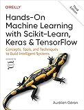
Hands-On Machine Learning with Scikit-Learn, Keras, and TensorFlow: Concepts, Tools, and Techniques to Build Intelligent Systems
- TRACK ML PROJECTS END-TO-END WITH SCIKIT-LEARN'S TOOLS.
- DISCOVER MULTIPLE MODELS: SVMS, TREES, FORESTS, AND ENSEMBLES.
- HARNESS ADVANCED NEURAL NETS FOR DIVERSE AI APPLICATIONS.


Designing Machine Learning Systems: An Iterative Process for Production-Ready Applications


The Hundred-Page Machine Learning Book (The Hundred-Page Books)


Why Machines Learn: The Elegant Math Behind Modern AI


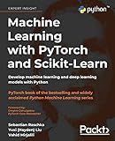
Machine Learning with PyTorch and Scikit-Learn: Develop machine learning and deep learning models with Python


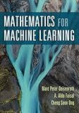
Mathematics for Machine Learning


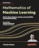
Mathematics of Machine Learning: Master linear algebra, calculus, and probability for machine learning


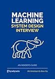
Machine Learning System Design Interview


The StatQuest Illustrated Guide To Machine Learning


Implementing a simple linear regression model in TensorFlow involves creating a computational graph that predicts a linear relationship between the input data and the output values. Here are the steps to implement the model:
- Import the necessary libraries: Import the TensorFlow library: import tensorflow as tf Import any other needed libraries, such as NumPy for data manipulation.
- Prepare the data: Load or create the input features (X) and output labels (y) datasets.
- Define the variables and placeholders: Create TensorFlow variables to store the trainable model parameters, usually called weights (W) and biases (b). Create TensorFlow placeholders to hold the input data (X) and output labels (y).
- Define the linear regression model: Create a TensorFlow operation that predicts the output using the formula y_pred = X * W + b.
- Define the loss function: Create a TensorFlow operation that calculates the loss between the predicted output (y_pred) and the actual output (y), such as mean squared error (MSE) or mean absolute error (MAE).
- Define the optimizer: Create a TensorFlow optimizer object (e.g., Gradient Descent, Adam) to minimize the loss function and update the model parameters.
- Train the model: Create a TensorFlow session to run the computational graph. Initialize the variables using tf.global_variables_initializer(). Use a loop to repeatedly feed the training data into the model, calculate the loss, and optimize the parameters. Optionally, validate the model's performance using validation data during training.
- Evaluate the model: Use the trained model to make predictions on new data. Calculate metrics such as mean squared error (MSE) or R-squared to evaluate the model's accuracy.
By following these steps, you can implement a simple linear regression model using TensorFlow to predict linear relationships between input features and output values.
How to update the model parameters using gradient descent?
To update the model parameters using gradient descent, you can follow these steps:
- Initialize the model parameters with random values.
- Calculate the gradient of the model parameters with respect to the loss function. This can be done by taking the derivative of the loss function with respect to each parameter.
- Update each parameter by subtracting the gradient multiplied by a learning rate. The learning rate determines how much the parameters are updated in each iteration. A smaller learning rate leads to slower convergence but more accurate results, while a larger learning rate leads to faster convergence but potentially less accurate results.
- Repeat steps 2 and 3 for a certain number of iterations or until convergence is reached. Convergence can be determined by monitoring the change in the loss function or the parameters in each iteration and stopping when it falls below a certain threshold.
In mathematical terms, the update rule for each parameter (θ) in gradient descent is:
θ_new = θ_old - learning_rate * gradient
Where θ_new is the updated parameter value, θ_old is the current parameter value, learning_rate is the learning rate, and gradient is the gradient of the parameter with respect to the loss function. The gradient can be positive or negative, so subtracting it from the parameter value adjusts the parameter in the direction that reduces the loss function.
What is the purpose of backpropagation in TensorFlow?
The purpose of backpropagation in TensorFlow is to update the weights and biases of a neural network during the training process. It is a method for computing the gradient of the loss function with respect to the trainable variables, which allows for the adjustment of these variables in the direction that minimizes the loss. By iteratively applying backpropagation, TensorFlow can optimize the parameters of the network and improve its performance over time.
How to implement forward propagation in a linear regression model?
To implement forward propagation in a linear regression model, you can follow these steps:
- Initialize the parameters: Start by initializing the weight matrix (W) and the bias (b) with small random values. The weight matrix will have dimensions (n x m), where n is the number of features and m is the number of output values.
- Perform the linear transformation: Compute the linear equation by multiplying the input features (X) with the weight matrix (W) and adding the bias (b). This can be represented as Z = X * W + b, where Z is the linear output.
- Apply activation function (optional): If necessary, you can apply an activation function such as ReLU or sigmoid to the linear output Z to introduce non-linearity. However, in linear regression, an activation function is not typically used.
- Compute the predicted output: The output of the forward propagation is the final prediction (y_hat). This can be obtained by using Z directly or by applying a specific function, depending on your problem.
- Calculate the loss: Compute the loss function by comparing the predicted output (y_hat) with the actual output (y). The most common loss function for linear regression is the mean squared error (MSE), which can be computed as the average of the squared differences between y and y_hat.
- Optional: Regularization. You can include regularization terms (such as L1 or L2 regularization) in the loss function to prevent overfitting.
Overall, the main steps are initializing parameters, performing the linear transformation, applying an optional activation function, computing the predicted output, calculating the loss, and optionally adding regularization.
How to split the dataset into training and testing sets?
There are several ways to split a dataset into training and testing sets. The most common methods are:
- Holdout method: This involves randomly dividing the dataset into two sets – a training set and a testing set. A common split ratio is 70% for the training set and 30% for the testing set.
- Cross-validation: Cross-validation involves creating multiple splits of the dataset into training and testing sets. One common approach is k-fold cross-validation, where the dataset is divided into k equal-sized subsamples. The model is trained on k-1 subsamples and tested on the remaining subsample, repeating the process k times with different subsamples.
- Time-based splitting: If the dataset contains a time dimension, it is important to split the data in a way that preserves the temporal order. For example, the training set can contain data up until a specific date, and the testing set can include data after that date.
- Stratified splitting: Stratified splitting is used when the dataset is imbalanced and you want to ensure that the training and testing sets have proportional representation of each class. This is especially important in classification tasks. The dataset is divided in a way that maintains the class distribution in both sets.
When splitting the dataset, it is important to maintain the randomization and reproducibility of the split. Most machine learning frameworks and libraries provide functions or methods for easy dataset splitting, such as scikit-learn's train_test_split() function.
What is the concept of underfitting and overfitting in TensorFlow?
Underfitting and overfitting are phenomena in machine learning, including the use of TensorFlow.
Underfitting refers to a situation where a model has not learned the underlying patterns in the data, resulting in poor performance on both the training and testing datasets. This occurs when the model is too simple or lacks the necessary complexity to capture the relationships within the data. An underfit model may have high bias and low variance.
Overfitting, on the other hand, occurs when a model learns the training data too well and fails to generalize to new, unseen data. It happens when the model becomes too complex or has too much capacity, capturing noise or random fluctuations in the training data. An overfit model may have low bias but high variance.
Both underfitting and overfitting lead to poor generalization, where the model struggles to accurately predict on unseen data.
To mitigate underfitting, one can consider increasing the model's complexity, such as adding more layers, neurons, or features. Additionally, adjusting hyperparameters, such as learning rate or regularization strength, can help improve performance.
To combat overfitting, techniques like regularization (e.g., L1 or L2 regularization), dropout, or early stopping can be utilized. Regularization imposes a penalty on the model's complexity, preventing it from over-emphasizing specific features. Dropout randomly deactivates some neurons during training, reducing over-dependence on individual neurons. Early stopping stops training when the model's performance on the validation set starts to deteriorate.
Striking the right balance between model complexity and generalization is crucial in TensorFlow (or any other machine learning framework) to achieve optimal performance on unseen data.
